Understanding Neural Networks: The Secret Lies in Our Brains
Reading is something I can guarantee you can do.
It’s something that comes naturally to us, from the long reports that we drudge on through to the short grocery lists we read every weekend.
On the other hand, machine learning algorithms have incredible capabilities, they can detect fraud, pilot autonomous vehicles, and interpret data at much higher speeds than our brain. Yet, getting programs to understand a simple handwritten text has puzzled many minds for almost half a century.
So, it was only logical to look towards what could understand things like text, our brains! Our brain is a highly complex information processing system, with a wide range of behaviors (some incredible like natural language, and some on the other end of the spectrum like indulging on that tenth chocolate bar).

Image recognition and natural language processing are both previously weak points of AI, with neural networks this has changed. Neural networks take inspiration from the neurons and behaviors of our brain (minus the chocolate), they’re a type of program composed of many artificial neurons chained together to generate complex behaviors.
A single neuron on its own is quite lacking with only a simple set of instructions. On the other hand, connected the system’s behavior becomes more complex.
Note: The behavior of a system relies on the structure of the neurons.
Neural networks have a few key features:
Information Processing 📁
In traditional cases, the information is processed in a CPU (central processing unit) which can only complete one task at a time. On the other hand, neural networks are composed of a combination of neurons that all process information individually.
Storing Data 📚
Within a computer, data storage is handled by the memory and processing is taken care of by the CPU. Within neural networks neurons both process and store data.
Data can be stored in two ways:
- Short term — stored within the neuron
- Long term — stored within the weights (channels connecting each neuron)
How a Neural Network Works 📝
All neural networks have neurons structured in the input, hidden, or output layers.

Input Layer is the layer receiving the input data and delivering it to the rest of the neural network.
Hidden Layer receives the data from the input nodes and they multiply it by a value called weights and add a value called the bias. (The whole network relies on adjusting weights and biases to generate the most accurate output possible. )
Output Layer is the final layer that assesses the information and calculates the output or resulting label.
In its simplest form, it’s an algorithm drawing lines to divide and categorize data. To sum it up, they learn relationships between the data inputted and the label outputted.
Finding the right line
Let’s start with a simple example where we’re drawing a straight line.
We can give our model a data set of inputs with the GPA of a student, and their ACT scores. Using this data we can try to predict whether or not a student got into Harvard. What the perceptron does is, to plot out each student as a point on a graph with the x coordinate as their GPA, and their y coordinate as their ACT score. What we can train the perception to do is to find a line where students above got accepted by Harvard and those below got rejected.
Graphing Lines
First, let’s understand how a single neuron operates. The neuron tries to model a linear relationship between two variables (their GPA and ACT scores in this case) using linear regression. This line model equation is a throwback to grade 9…
y = mx + b
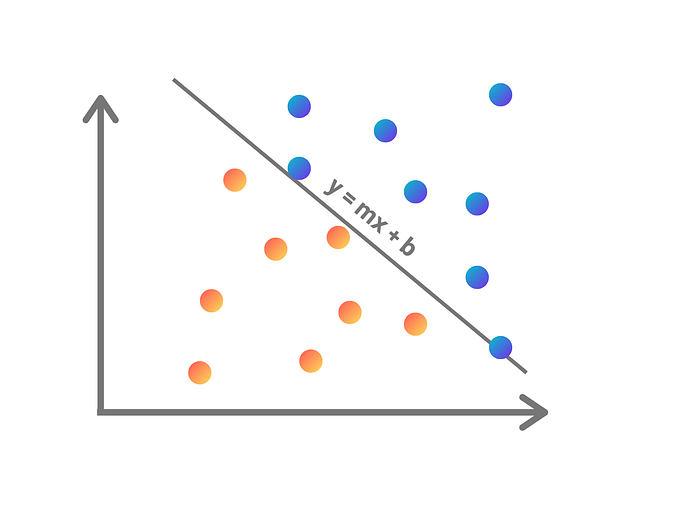
This goal of this line is to separate the students who got accepted vs who got rejected as best as possible. You can also look at the line as the equal point where you’re equally likely to be accepted and rejected.
Understanding the Perceptron 🎓
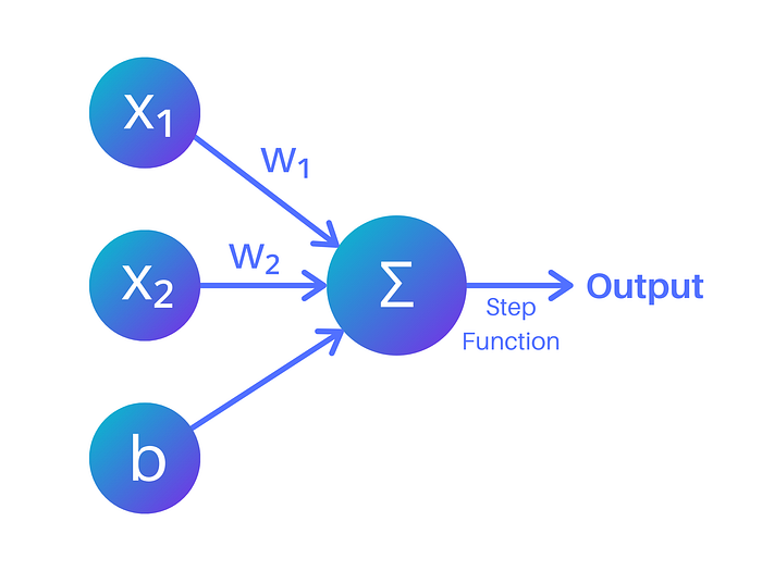
Now let’s zoom in on a perceptron. A perceptron is a type of neural network with a single layer, they are linear classifiers. A perceptron takes in multiple inputs, in our case we have two the GPA and ACT scores. These inputs (x) are multiplied by a weight (w). If it’s easier to imagine you can think of weights as the strength of a connection between neurons. After the inputs are multiplied with their corresponding weight, they are summed together and a bias is added (usually the bias also has its own weight that it’s multiplied by).
Here’s the general form:
w₁x₁ + w₂x₂ + b = 0
Here’s the general form simplified:
y = mx + b
Activation Function
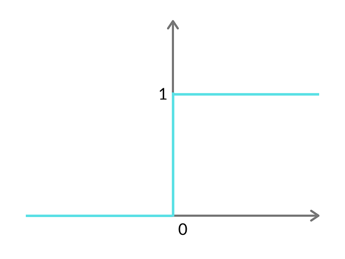
Then we need to pass it through an activation function that defines the output of the neuron. In our case, we are going to start with the step activation function.
The prediction (ŷ):
ŷ = 1 if wx + b >= 0
ŷ = 0 if wx + b < 0
In actual words, this means that is the equation calculated to above or equal to 0 the algorithm will predict True, otherwise it will predict False.
Note: Y hat (ŷ) stands for the predicted value of y (the dependent variable in our case whether or not the student was accepted)
Side Note: If you go deeper into neural networks you’ll learn about the sigmoid function which transforms a value into a number from 0 to 1.
Error
The error that we are programming today is the difference between the correct label and what our algorithm predicted.
error_Value = label — output
Later on, you can also learn to calculate error using gradient descent, which moves in the direction of the steepest descent. In other words, how far away the algorithm is from the correct label determines the extent of the change to the algorithm.
Learning Rate
So now that you have an error value we can readjust the line equation to correctly classify more points. So we can input the values of the misclassified point in this equation as x to correct the weights, which in turn adjust the line.
new_Weights = previous_Weights + (x * error_Value * learning_Rate)
Now you might be wondering what the learning rate is. The learning rate is there to prevent huge changes to the line. If you had one outlier point and changed the entire line to correctly classify that point, you would end up with a lot more incorrectly classified points than before.
Putting it all together
Here we can see the inputs multiplied by the weights and added with the bias. The step function is then applied to generate a predicted output, this process of propagating information through the network is known as forward propagation.
Then, we look at the points multiplied by the error and learning rate to create better more accurate weights. (If you used gradient descent to calculate the error, this process of sending data back through the network is known as backpropagation.)
Coding it in Python 💻
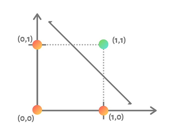
Now let’s start by coding a perceptron. We’re going to code the AND logical operator, it’s not the most practical but it is quite straightforward and good for explaining the basics of neural networks.

The AND logical operator only returns true when both inputs are true.
First, we take the two possible inputs, True or False and transform them into binary…
This is the same data we’ll later use to train the algorithm.
The algorithm we’ll program simply predicts the end output base on the two inputs.
Here we plotted out the different possible inputs as points in a graph, what we aim to formulate is the line that separates the different colored points.
Setting the Variables
In our python program, we’ll start by defining the variables for the weights, the bias, and the learning rate.
# The AND logic gate coded as a neural network
# This perceptron is not the most efficient neural network but it's simple to code! It's a nice classifer for explaining concepts!import random
inputOne_Weights = random.random()#Let's randomly assign values
inputTwo_Weights = random.random()#We will adjust the weights later
bias_Weights = random.random()bias = 1
learning_Rate = 1 #usually it's a lot smaller but we have less data and it's a simple preceptron
Next, we’ll define a function that returns the output derived straight from the input, weights, and bias
def calcOutput (x,y):
 output = x*inputOne_Weights + y*inputTwo_Weights+bias*bias_Weights
 return output
Here, we’re defining the main perceptron. This is where we calculate the output, apply the activation function, and use the error to edit the weights accordingly.
# x and y are the two different inputs and the label is the correct result for each case
def perceptron (x, y, label):
  output = calcOutput(x,y)
  if output > 0:    output = 1  #Here comes the step function
  else:             output = 0
  errorValue = label - output  #find the error value# Adjust the weights according to the error value times the learning rate
# Make sure you edit the global variable (outside function)
  global inputOne_Weights
# Let's edit the weights according to the input, error, and learning rates
  inputOne_Weights += x * errorValue * learning_Rateglobal inputTwo_Weights
  inputTwo_Weights += y * errorValue * learning_Rateglobal bias_Weights
  bias_Weights += bias * errorValue * learning_Rate
After defining the perceptron, we need to train it to better predict the correct outcome. This is just running through the perceptron with different data points over and over again.
def training (epoch): #epoch ~ is number of passes of training data
  for i in range(epoch):
    # Since an AND function only takes two inputs and two types of      values (0 or 1) there are only four pieces of data
    # Here's our test data! We're running it through the perceptron
    perceptron(0,0,0)
    perceptron(1,0,0)
    perceptron(0,1,0)
    perceptron(1,1,1)
Now we put all the functions together, we run through the entire program to see if our perception works.
def test (x,y):
  training(56)  # here we choose how many epochs
  output = calcOutput(x,y)
  if output > 0:    output = 1           # Here's our step function
  else:             output = 0
  return outputx = int(input())   # These are the two inputs
y = int(input())
print(test(x,y))     # Now let's run through the whole program and check if it works
Run the program and see if it works! Go through all the test cases and check if the program calculates the correct output.
Key Takeaways 📌
- Neural networks are inspired by the neurons and structure of our own brains, they are composed of neurons that each process information individually and pass it on throughout the network
- The neural network has a few key differences in information processing and how they store data, compared to traditional methods the neuron does both the processing and storing of data
- Neural networks are composed interconnected neurons that form of three different layers: input, hidden, and output
- The core principle of the algorithm is to separate and classify the data with a line (model a linear relationship using linear regression).
- A perceptron takes inputs multiplies them by the weights, adds the bias, and passes the sum through an activation function.
- The activation function we used was a binary step function, which means that if the input data is above a threshold (0 in our case) the neuron is activated and sends the data onwards to the next layer.
- The act of feeding the input data through the network passed from neuron to neuron is known as forward-propagation.
- Calculating the error and adjusting the weights to minimize it uses something called back-propagation. Where the output error is propagated backward to adjust the weights in each layer.
Phew, that was quite a long article! Congrats, now you have a better understanding of how a neural network operates and you’ve even coded one!
I hope this piqued your interest in neural networks and that you learned something interesting!
See that icon below, the one with the clap sign? Try clicking on it, go on try it! Confetti, cool right? If you want to read more articles in the future or like the confetti, give my account a follow!
In the meantime, feel free to contact me at ariel.yc.liu@gmail.com or connect on LinkedIn. You can also read my monthly newsletter here!
Till next time! 👋

